Checking Distribution for Continuous Variables Sas
Below is an example of code used to investigate the distribution of a variable. In our example, we will use the hsb2 data set and we will investigate the distribution of the continuous variable write, which is the scores of 200 high school students on a writing test. We use the plots option on the proc univariate statement to produce the stem-and-leaf and normal probability plots shown at the bottom of the output. We will start by showing all of the unaltered output produced by this command, and then we will annotate each section.
proc univariate data = "D:\hsb2" plots; var write; run;
The UNIVARIATE Procedure Variable: write (writing score)
Moments
N 200 Sum Weights 200 Mean 52.775 Sum Observations 10555 Std Deviation 9.47858602 Variance 89.843593 Skewness -0.4820386 Kurtosis -0.7502476 Uncorrected SS 574919 Corrected SS 17878.875 Coeff Variation 17.9603714 Std Error Mean 0.67023725
Basic Statistical Measures
Location Variability
Mean 52.77500 Std Deviation 9.47859 Median 54.00000 Variance 89.84359 Mode 59.00000 Range 36.00000 Interquartile Range 14.50000
Tests for Location: Mu0=0
Test -Statistic- -----p Value------
Student's t t 78.74077 Pr > |t| <.0001 Sign M 100 Pr >= |M| <.0001 Signed Rank S 10050 Pr >= |S| <.0001
Quantiles (Definition 5)
Quantile Estimate
100% Max 67.0 99% 67.0 95% 65.0 90% 65.0 75% Q3 60.0 50% Median 54.0 25% Q1 45.5 10% 39.0 5% 35.5 1% 31.0 0% Min 31.0
----------------------------------------------------------------
The UNIVARIATE Procedure Variable: write (writing score)
Extreme Observations
----Lowest---- ----Highest---
Value Obs Value Obs
31 89 67 118 31 40 67 160 31 39 67 177 31 31 67 183 33 70 67 185
Stem Leaf # Boxplot 66 0000000 7 | 64 0000000000000000 16 | 62 0000000000000000000000 22 | 60 00000000 8 +-----+ 58 0000000000000000000000000 25 | | 56 000000000000 12 | | 54 00000000000000000000 20 *-----* 52 0000000000000000 16 | + | 50 00 2 | | 48 00000000000 11 | | 46 00000000000 11 | | 44 0000000000000 13 +-----+ 42 000 3 | 40 0000000000000 13 | 38 000000 6 | 36 00000 5 | 34 00 2 | 32 0000 4 | 30 0000 4 | ----+----+----+----+----+
---------------------------------------------------------------------
The UNIVARIATE Procedure Variable: write (writing score)
Normal Probability Plot 67+ +++ ***** ** | ******* | ***** | **++ | ****+ | ***++ | ***++ | ***++ | **++ 49+ **+ | *** | *** | ++* | +*** | +** | +** | ++* | +*** 31+**+** +----+----+----+----+----+----+----+----+----+----+
Basic descriptive statistics
The UNIVARIATE Procedure Variable: write (writing score) Moments a N b 200 Sum Weights h 200 Mean c 52.775 Sum Observations i 10555 Std Deviation d 9.47858602 Variance j 89.843593 Skewness e -0.4820386 Kurtosis k -0.7502476 Uncorrected SS f 574919 Corrected SS l 17878.875 Coeff Variation g 17.9603714 Std Error Mean m 0.67023725
a. Moments – Moments are a statistical summaries of a distribution.
b. N – This is the number of valid observations for the variable. The total number of observations is the sum of N and the number of missing values. If there are missing values for the variable, proc univariate will output the statistics about the missing values, such as the number and the percentage of missing values.
c. Mean – This is the arithmetic mean across the observations. It is the most widely used measure of central tendency. It is commonly called the average. The mean is sensitive to extremely large or small values.
d. Std Deviation – Standard deviation is the square root of the variance. It measures the spread of a set of observations. The larger the standard deviation is, the more spread out the observations are.
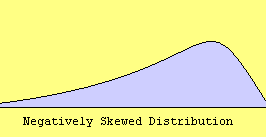
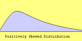
e. Skewness – Skewness measures the degree and direction of asymmetry. A symmetric distribution such as a normal distribution has a skewness of 0, and a distribution that is skewed to the left, e.g. when the mean is less than the median, has a negative skewness.
f. Uncorrected SS – This is the sum of squared data values. The two summations: sum of observations and sum of squares are related to the calculation of variance in the following way:
Variance= (sum of squares -(sum of observations)2/N)/(N-1)
g. Coeff Variation – The coefficient of variation is another way of measuring variability. It is a unitless measure. It is defined as the ratio of the standard deviation to the mean and is generally expressed as a percentage. It is useful for comparing variation between different variables.
h. Sum Weights – A numeric variable can be specified as a weight variable to weight the values of the analysis variable. The default weight variable is defined to be 1 for each observation. This field is the sum of observation values for the weight variable. In our case, since we didn't specify a weight variable, SAS uses the default weight variable. Therefore, the sum of weight is the same as the number of observations.
i. Sum Observations – This is the sum of observation values. In case that a weight variable is specified, this field will be the weighted sum. The mean for the variable is the sum of observations divided by the sum of weights.
j. Variance – The variance is a measure of variability. It is the sum of the squared distances of data value from the mean divided by the variance divisor. The variance divisor is defined to be either N-1 or N controlled by the option vardef. The default option is vardef=df, which is N-1. The Corrected SS is the sum of squared distances of data value from the mean. Therefore, the variance is the corrected SS divided by N-1. We don't generally use variance as an index of spread because it is in squared units. Instead, we use standard deviation.
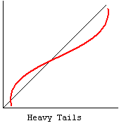
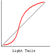
k. Kurtosis – Kurtosis is a measure of the heaviness of the tails of a distribution. In SAS, a normal distribution has kurtosis 0. Extremely nonnormal distributions may have high positive or negative kurtosis values, while nearly normal distributions will have kurtosis values close to 0. Kurtosis is positive if the tails are "heavier" than for a normal distribution and negative if the tails are "lighter" than for a normal distribution. Please see our FAQ on kurtosis What's with the different formulas for kurtosis?
l. Corrected SS – This is the sum of squared distance of data values from the mean. This number divided by the number of observations minus one gives the variance.
m. Std Error Mean – This is the estimated standard deviation of the sample mean. If we drew repeated samples of size 200, we would expect the standard deviation of the sample means to be close to the standard error. The standard deviation of the distribution of sample mean is estimated as the standard deviation of the sample divided by the square root of sample size. This provides a measure of the variability of the sample mean. The Central Limit Theorem tells us that the sample means are approximately normally distributed when the sample size is 30 or greater.
More basic statistics
Basic Statistical Measures Location Variability Mean 52.77500 Std Deviation 9.47859 Median n 54.00000 Variance 89.84359 Mode o 59.00000 Range p 36.00000 Interquartile Range q 14.50000
n. Median – The median is a measure of central tendency. It is the middle number when the values are arranged in ascending (or descending) order. Sometimes, the median is a better measure of central tendency than the mean. It is less sensitive than the mean to extreme observations.
o. Mode – The mode is another measure of central tendency. It is the value that occurs most frequently in the variable. It is used most commonly when the variable is a categorical variable.
p. Range – The range is a measure of the spread of a variable. It is equal to the difference between the largest and the smallest observations. It is easy to compute and easy to understand. However, it is very insensitive to variability.
q. Interquartile Range – The interquartile range is the difference between the upper and the lower quartiles. It measures the spread of a data set. It is robust to extreme observations.
Tests of location
Tests for Location: Mu0=0 Test r -Statistic- s -----p Value------ t Student's t u t 78.74077 Pr > |t| <.0001 Sign v M 100 Pr >= |M| <.0001 Signed Rank w S 10050 Pr >= |S| <.0001
r. Test – This column lists the various tests that are provided.
s. Statistic – This column lists the values of the test statistics.
t. p Value – This column lists the p-values associated with the test statistics.
u. Student's t – The Student t-test is used to test the null hypothesis that the population mean equals Mu0. The default value in SAS for Mu0 is 0. The t-statistic is defined to be the difference between the mean and the hypotheses mean divided by the standard error of the mean. The p-value is the two-tailed probability computed using a t distribution. If the p-value associated with the t-test is small (usually set at p < 0.05), there is evidence to reject the null hypothesis in favor of the alternative. In other words, the mean is statistically significantly different than the hypothesized value. If the p-value associated with the t-test is not small (p > 0.05), the null hypothesis is not rejected. In our example, our t-value is 78.74077 and the corresponding p-value is less than 0.0001. We conclude that there is a statistically significant difference between the mean of the variable write and zero.
v. Sign – The sign test is a simple nonparametric procedure to test the null hypothesis regarding the population median. It does not require that the sample is drawn from a normal distribution. It is used when we have a small sample from a nonnormal distribution. The statistic M is defined to be M=(N+-N–)/2 where N+ is the number of values that are greater than Mu0 and N– is the number of values that are less than Mu0. Values equal to Mu0 are discarded. Under the hypothesis that the population median is equal to Mu0, the sign test calculates the p-value for M using a binomial distribution. The interpretation of the p-value is the same as for t-test. In our example the M-statistic is 100 and the p-value is less than 0.0001. We conclude that the median of variable write is significantly different from zero.
w. Signed Rank – The signed rank test is also known as the Wilcoxon test. It is used to test the null hypothesis that the population median equals Mu0. It assumes that the distribution of the population is symmetric. The Wilcoxon signed rank test statistic is computed based on the rank sum and the numbers of observations that are either above or below the median. The interpretation of the p-value is the same as for the t-test. In our example, the S-statistic is 10050 and the p-value is less than 0.0001. We therefore conclude that the median of the variable write is significantly different from zero.
Quantiles
Quantiles (Definition 5) Quantile Estimate 100% Max x 67.0 99% 67.0 95% y 65.0 90% 65.0 75% Q3 z 60.0 50% Median 54.0 25% Q1 bb 45.5 10% 39.0 5% 35.5 1% 31.0 0% Min cc 31.0
x. 100% Max – This is the maximum value of the variable. One hundred percent of all values are equal to or less than this value.
y. 95% – Ninety-five percent of all values of the variable are equal to or less than this value.
z. 75% Q3 – This is the third quantile. Seventy-five percent of all values are equal to or less than this value.
bb. 25% Q1 – This is the first quantile. Twenty-five percent of all values of the variable are equal to or less than this value.
cc. 0% Min – This is the minimum value. Zero percent of values are less than this value.
Extreme values, stem-and-leaf plot and boxplot
The UNIVARIATE Procedure Variable: write (writing score) Extreme Observations ee ----Lowest---- ----Highest--- Value Obs Value Obs 31 89 67 118 31 40 67 160 31 39 67 177 31 31 67 183 33 70 67 185 Stem Leaf ff # Boxplot gg 66 0000000 7 | 64 0000000000000000 16 | 62 0000000000000000000000 22 | 60 00000000 8 +-----+ z 58 0000000000000000000000000 25 | | 56 000000000000 12 | | 54 00000000000000000000 20 *-----* aa 52 0000000000000000 16 | + | c 50 00 2 | | 48 00000000000 11 | | 46 00000000000 11 | | 44 0000000000000 13 +-----+ bb 42 000 3 | 40 0000000000000 13 | 38 000000 6 | 36 00000 5 | 34 00 2 | 32 0000 4 | 30 0000 4 | ----+----+----+----+----+
ee. Extreme Observations – This is a list of the five lowest and five highest values of the variable.
ff. Stem Leaf – The stem-leaf plot is used to visualize the overall distribution of a variable. In this display, the stem is the portion of the value to the left and the leaf is the part to the right. The number on the right is the number of leaves on each stem. For example, one the first line, the stem is 66, and there are seven 0's to the right of this stem, indicating that there are seven cases with a value of 66 or 67 for this variable.
gg. Boxplot – The box plot is a graphical representation of the 5-number summary for a variable. It is based on the quartiles of a variable. The rectangular box corresponds to the lower quartile and the upper quartile. The line in the middle is the median. The plus sign in the middle is the mean. We can visually compare the lengths of the whiskers. If one is clearly longer than the other one, the distribution may be skewed.
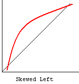
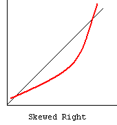
The UNIVARIATE Procedure Variable: write (writing score) Normal Probability Plot cc 67+ +++ ***** ** | ******* | ***** | **++ | ****+ | ***++ | ***++ | ***++ | **++ 49+ **+ | *** | *** | ++* | +*** | +** | +** | ++* | +*** 31+**+** +----+----+----+----+----+----+----+----+----+----+ cc. Normal Probability Plot – The normal probability plot is used to investigate whether the variable is normally distributed. The plus signs in the plot indicate a normal distribution, and they form a straight line. The asterisks show the data values. If our variable is close to normal distribution, then the asterisks will also be close to a straight line and thus cover most of the plus signs. There are different types of departure from normality, some examples of which are shown below.
References
- S. Schlotzhauser and R. Littell, SAS System for Elementary Statistical Analysis, 2nd Edition, Cary, NC: SAS Institute Inc., 1997.
Source: https://stats.oarc.ucla.edu/sas/output/proc-univariate/
0 Response to "Checking Distribution for Continuous Variables Sas"
Post a Comment